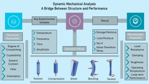
Figure 1: Graphical Abstract

1. Introduction

Dynamic Mechanical Analysis (DMA) has emerged as a central technique for evaluating the viscoelastic behavior of materials, especially polymers. Its importance becomes clear when recognizing that a material’s performance can shift drastically between manufacturing conditions and real service environments. A well-known historical example is the failure of the Titanic’s hull steel, which became extremely brittle in cold seawater despite showing acceptable ductility at room temperature [1]. This mismatch between testing temperature and operating conditions contributed to catastrophic fracture, underscoring why temperature-dependent mechanical characterization is critical for ensuring reliability.

DMA provides this capability by measuring how stiffness, damping, and mechanical transitions evolve with temperature, frequency, and strain. Originally developed to study simple metallic wires, the technique has expanded significantly as instrumentation improved. As outlined by Menard in Dynamic Mechanical Analysis: A Practical Introduction [2]. In the field of polymer applications, DMA enables to direct observation on different structural properties like molecular mobility, chain orientations, glass transition, secondary relaxations, crosslink density, filler–matrix interactions, and morphological evolution. These insights cannot be obtained from static mechanical tests alone and often correlate strongly with real-world performance such as impact resistance, dimensional stability, and fatigue behavior.

In recent years, Dynamic Mechanical Analysis (DMA) has proven its value in elucidating polymer behavior under various conditions. For example, a 2025 study on fluorinated-polyurethane coatings showed DMA could track how long-term environmental exposure shifts the glass-transition temperature (T_g), alters elastic modulus (E′), and changes relaxation behavior — offering insight into degradation, crosslink changes, and moisture-induced plasticization over years of outdoor use [3]. Another recent work on a 50/50 blend of isotactic polypropylene (iPP) and polyamide 6 (PA6) used DMA to investigate how different interfacial agents influence miscibility, blend morphology, and mechanical response under oscillatory stress; the results revealed clear differences in storage modulus and transition behavior depending on compatibilization strategy [4].

Because DMA provides rapid, sensitive, and structure-dependent mechanical data, it has evolved into an indispensable tool for polymer development and quality control. It supports design optimization, failure analysis, and durability assessment — by linking molecular structure, processing conditions, environmental exposure, and mechanical performance in a single coherent framework.

2. Fundamentals of DMA:

Understanding DMA begins with the foundations of mechanical behavior—specifically how materials respond to stress and strain. When an external force is applied, a material deforms, and the relationship between the applied stress (σ) and resulting strain (ε) describes its mechanical properties. In DMA, this stress-strain behavior is observed at different temperatures or frequency. For the elastic component where under the elastic limit, complete recoverable deformation is observed. Crystallinity is the main cause of the elasticity where Intermolecular force > applied force.

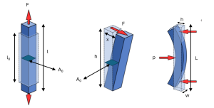
If a solid of constant cross section A₀ and an initial length l₀ is subjected to a tensile force F, it will deform in the direction of the force, as shown in Figure.

The stress σ, having units of force per area, is defined as σ = F /A₀ 

If l is the length of the sample, the engineering strain ε, having units of length per length, is defined as ε = (l-l₀) /l₀

An ideal solid may be defined as a material in which strain is proportional to stress in conformance to Hooke’ s law: σ = Eε

Where E is the elastic modulus or Young’s modulus.  In case of shear force, if the cross section of a body is A₀, applied force is F and horizontal displacement is x and height is h. The equation of the shear stress τ = F /A₀ and shear strain is γ = x/h

In case of flexural mode of deformation, three – point bending test is done. For a sample of length L, width w,

and thickness h, loaded as shown in the figure with a load P , the flexural modulus (E_f), is defined by: E_f = (L³P)/(4wh³δ)

Where δ is the linear deflection at the point of loading.

For viscous components when force is applied it causes the permanent deformation, as the amorphous content is the majority in viscous material. Here the intermolecular force is < applied force. The polymer exhibits both elastic property and viscous property. In combination polymers can be said as viscoelastic material and it shows viscoelasticity (both elastic and viscous property) at different temperatures. The main objective of DMA is to observe this viscoelastic behavior. DMA involves applying a sinusoidal strain (or stress) to a sample and measuring the corresponding stress (or strain) developed. Both approaches are theoretically identical. Consider what happens if a sinusoidal strain is applied to an ideal elastic solid: ε(t) = ε₀ sin (ωt)

At any point in time the stress will be proportional to the strain in accordance with Hooke ’ s law: σ(t) = Eε(t) = E ε₀ sin⁡(ωt) = σ₀ sin⁡(ωt)

where ε₀ is the strain amplitude and is the angular frequency. The resulting stress response is also sinusoidal but lags behind the applied strain by a phase angle:

σ(t)=σ₀ sin⁡(ωt+δ)

Thus, for an ideal solid the stress will be a sinusoidal function in phase with the strain, as shown in Fig 2. and the ratio of amplitudes of stress and strain will be the modulus of the material: E = σ₀ / ε₀ 

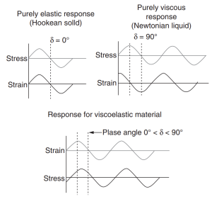
Figure 2: Elastic, Viscose and Viscoelastic material response [5]

From the sinusoidal response, DMA separates the material’s behavior into two measurable components:

• Storage Modulus (E′) – Represents the elastic portion of the response. It is a measure of the elastic character or solid like nature of the material. It indicates how much mechanical energy is stored per cycle and returned upon unloading. High E′ values correspond to stiff, glassy behavior. It is defined as: E’ = (σ₀ε₀)/ cos⁡δ
• Loss Modulus (E″) – E″ is known as the loss modulus and is a measure of the viscous character or liquidlike nature of the material. It represents energy dissipated as heat and is often used to detect molecular relaxations, transitions, or the onset of flow. For an ideal elastic solid, the phase lag is zero. Thus, E′ is simply Young ’ s modulus of the material and E″ is zero. For an ideal viscous liquid the phase lag is 90 °. Quantifies the viscous portion of the response: E” = (σ₀/ε₀)/ sin⁡δ
• Loss Tangent or Damping factor (tan δ) – The ratio of viscous to elastic response: tan⁡δ = E” / E’

3. Experimental Setup & Methodology

A successful DMA experiment relies on careful specimen preparation, proper instrument setup, and precise control of test conditions. Because DMA is highly sensitive to geometry, temperature, and loading history, even small deviations can significantly influence the measured viscoelastic response. This section outlines the essential steps and considerations required to obtain reliable and interpretable data. Schematic of a DMA is shown in figure 3 [2].

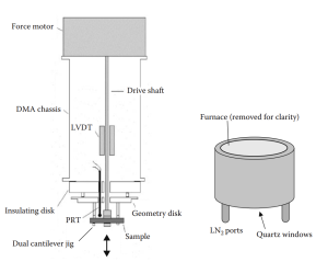
Figure 3: Schematic of the PerkinElmer DMA 8000 showing the motor, Linear Vertical
Displacement Transducer (LVDT), sample compartment, furnace, and heat sink. [2]

3.1 Sample Preparation: DMA requires specimens with well-defined geometry, uniform thickness, and smooth surfaces. Errors in dimensions directly impact calculated modulus values, as modulus is normalized by sample geometry. Rectangular bars, films, fibers, disks, or small molded parts can be tested depending on the fixture. Polymers must also be conditioned prior to testing to minimize moisture effects, as water acts as a strong plasticizer. For thermosets or composites, post-curing may be required to ensure the sample reflects its intended final state.

3.2 Selection of Deformation Mode: Different fixtures allow DMA to be applied to a broad range of materials. Clamps for different test method is shown figure 4 collected from [6]

• Three-point bending or dual cantilever – Ideal for stiff or very stiff materials, rigid polymers and composites.
• Tension mode – Used for films, fibers, thin laminates, bar, or ductile polymers.
• Compression mode – Used for foams, gels, or soft solids.
• Shear or torsion – Preferred for polymers, elastomers, adhesives, and rubber-like materials.

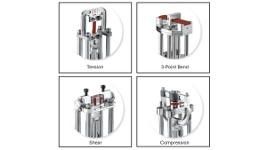
Figure 4: Schematic of different types of clamps [6].

3.3 Instrument Configuration: A DMA instrument applies an oscillatory load while precisely controlling temperature. The furnace or environmental chamber must be calibrated to ensure uniform heating, as temperature gradients can shift transition temperatures. Clamp alignment is equally critical—misalignment introduces bending in tension tests or shear in bending tests, distorting results. Many modern DMA instruments include automatic tensioning systems to prevent preloading errors that can artificially increase stiffness.

3.4 Test Variables and Scanning Methods: DMA instruments operate by applying a dynamic (oscillating or pulsing) force to a sample and analyzing the resulting material response (strain). The experimental methodology focuses on precisely controlling four primary variables:

1. Stress/Strain Control (Amplitude): DMA instruments can operate under stress (force) control or strain (displacement) control. a) Strain-controlled analyzers move the probe a set distance and measure the resulting stress with a load cell. They often have better short-time response for low viscosity materials. b) Stress-controlled analyzers apply a set force and are often considered to duplicate real-life conditions more accurately since most polymer applications involve resisting a load. DMA tests are generally run at very low strains (e.g., $\le 0.5\%$) to ensure the material remains within the linear viscoelastic region (LVR). A dynamic strain sweep is used to determine this LVR by continually increasing the amplitude (strain or stress) at a fixed rate.
2. Temperature (T): Temperature is a critical variable because material properties are strongly influenced by it. Temperature control involves a furnace, a heat sink, and a temperature measuring device (often a thermocouple). The system must be calibrated, ideally using NIST traceable materials like indium or tin. For testing to be accurate, temperature control must be accurate and reproducible. Large samples are discouraged because they can lead to thermal lags and anomalies, requiring very slow heating rates. Temperature programs can include simple ramps, or complex cycles with ramps and isothermal holds, to simulate environmental thermal cycles or process conditions.
3. Frequency ($\omega$ or $f$): Frequency is the rate of oscillation of the applied dynamic stress. Frequency effects are typically studied by performing a frequency scan, where the temperature is held constant while the frequency is varied. Alternatively, data can be collected in a multiplex by applying a set of frequencies while ramping the temperature. To compensate for the limited frequency range of instruments, data may be added from creep experiments (providing results at very low strain rates) or free resonance studies (providing results at higher rates of deformation)
4. Time ($t$): Time is the duration of testing, primarily controlled during isothermal studies or non-dynamic tests performed on DMA instruments. Creep-Recovery Testing involves applying a constant static load (creep step) and observing the resulting deformation over time, followed by removing the load to monitor recovery. Stress Relaxation Experiments involve deforming a sample to a set length and measuring the decay of the stress exerted by the sample over time. Time-based studies are essential for curing studies (monitoring changes in viscosity/modulus over time), as well as long-term performance prediction and aging (often using superposition principles). 

4. Data Interpretation Peer-Reviewed Paper

4.1 Temperature-sweep curves: the basic picture: In most polymer studies, DMA data are presented as storage modulus (E′), loss modulus (E″), and loss factor (tan δ) plotted against temperature or frequency. A single well-designed experiment can already show glass transition, secondary relaxations, crosslink density trends, filler effects, and miscibility.

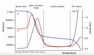
Figure 5: Typical DMA Outputs for Polymers

In a standard temperature sweep at fixed frequency and strain, three curves are obtained: E′(T) or G′(T) , E″(T) or G″(T), and tan δ(T). For a typical thermoplastic, E′ is high and almost constant in the glassy region at low temperature, then drops steeply through the glass-transition region, and finally levels off into a rubbery plateau at higher temperature. E″ and tan δ show peaks in the transition region, where molecular mobility increases and energy dissipation is highest. These features allow user to identify service windows: glassy and stiff at low T, rubbery and flexible at intermediate T, and flowing or softening at very high T. One of the important feature of the DMA is to able to determine the glass transition temperature.

4. 2: Glass transition and secondary relaxations:  The glass transition (T_g) can be taken from several DMA signals:

• Onset of the drop in E′

• Peak in E″

• Peak in tan δ

In practice, many authors use either the E″ peak or tan δ peak because they are easier to locate than an onset on E′, especially for noisy data. Smaller peaks or shoulders at lower temperatures are often assigned to secondary relaxations (β, γ, etc.), which correspond to local side-group motions or restricted segmental motions. These are important for impact resistance, damping, and low-temperature toughness.

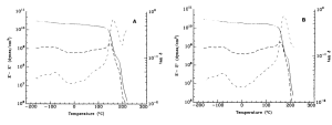
Figure 6: The DMA properties of HPMC (Hydroxypropyl methylcellulose) in (Left: Average Mw: 3000, Right: Average Mw: 6000) Here (—) storage modulus E′, (light dash –) loss modulus E″, (dark dash –) tan δ [7]

The results from the DMA analysis of the HEC film are shown in Figure 6. This polymer also showed primary and
secondary transitions similar to those seen with HPMC. For lower molecular weight polymer, primary transition showed in 160º and for higher molecular weight of polymer primary transition showed in 175º. The secondary transition showed at -40 to -150 and 50 to 100 for both lower and higher molecular weight of HPMC. The secondary transition refers to the movement of the side chain.

4. 3: Post curing process analysis: DMA can be used to analysis the mechanical performance of the polymer after curing process. To obtain the optimal curing parameter, multiple DMA test is done. After evaluation DMA shows the optimal curing process that provides the best performance.

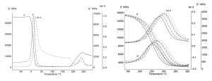
Figure 7: Left (storage modulus E′, loss modulus E″, tan δ of carbon fiber epoxy prepreg before curing), Right (DMA results for fully cured prepreg during cooling from the maximum temperature) [8]

The sources indicate that the properties of the carbon fibre epoxy prepreg improved (increased stiffness) after curing, primarily evidenced by a significant increase in the material’s Glass Transition Temperature (T_g​) and, consequently, its mechanical stability at higher temperatures. 

• Before Curing: The uncured material exhibited a glass transition (T_g0​) near 1^∘C. This transition causes a sharp drop in the storage modulus (E′), meaning the material loses stiffness rapidly just above this temperature.
• After Curing: The fully cured material exhibits a maximal glass transition temperature (T_gmax​) in the range of 220^∘C to 230^∘C.

The experiment that produced Figure 7 (Right) involved an immediate cooling run applied to the sample after it had completed the 1 K/min heating run up to the maximum temperature of 280^∘C. The intention of this test was to investigate the mechanical properties of the sample under the same clamping conditions to allow for a direct comparison between the uncured and cured material. 

5. Application

Dynamic Mechanical Analysis (DMA) is widely used across polymer science and engineering because it connects molecular-level mobility with real mechanical performance. One of its most common applications is determining the glass-transition temperature (T_g), which marks the shift from a hard, glassy polymer to a softer, rubbery one. This helps engineers understand how a polymer will behave in different environments.

DMA is also important for evaluating crosslink density and cure state in thermosets and elastomers. By looking at the rubbery-plateau modulus, researchers can estimate how tightly the polymer network is crosslinked, which influences stiffness, toughness, and long-term stability. This makes DMA a key tool for curing optimization and quality control.

For polymer blends and composites, DMA provides sensitive information about phase compatibility. Miscible blends typically show a single tan δ peak, while immiscible blends display two or more transitions. Composites containing fillers or nanofillers often exhibit increased storage modulus and changes in damping behavior. These shifts show how additives restrict chain mobility and modify the material’s mechanical response.

In addition, DMA is commonly used to measure damping and dynamic loading performance, especially for elastomers, impact-resistant materials, and vibration-isolating components. Loss modulus (E″) and tan δ curves help designers select materials for applications involving repeated or high-frequency loading.

DMA is also valuable in failure analysis, durability assessment, and quality assurance. Because it measures mechanical behavior as a function of temperature, time, and frequency, DMA helps identify early signs of degradation, improper processing, or inconsistencies between batches. This makes it an essential characterization tool for industries ranging from aerospace to biomedical polymers.

6. Conclusion

DMA provides a powerful and versatile framework for understanding how polymers behave under realistic mechanical and environmental conditions. By separating elastic and viscous responses, DMA reveals transitions, relaxation mechanisms, and structural changes that are often invisible in conventional mechanical tests. Its sensitivity to temperature, frequency, and molecular mobility makes it uniquely equipped to link polymer chemistry and microstructure with practical performance. Whether used to fine-tune material formulations, predict service behavior, or diagnose failures, DMA stands as a key method in modern polymer characterization and continues to support innovation across research and industry.

References

1. Causes and effects of the rapid sinking of the titanic, [Online; accessed 2025-12-09]. URL https://writing.engr.psu.edu/uer/bassett.html
2. Menard, K. P., & Menard, N. (2020). Dynamic mechanical analysis. CRC press.
3. Startsev, O. V., Mastalygina, E. E., Vetcher, A. A., Koval, T. V., Veligodsky, I. M., Dvirnaya, E. V., & Iordanskii, A. L. (2025). Long-Term Environmental Aging of Polymer Composite Coatings: Characterization and Evaluation by Dynamic Mechanical Analysis. Journal of Composites Science, 9(12), 645.
4. Collar, E. P., & García-Martínez, J. M. (2024). A Dynamic Mechanical Analysis on the Compatibilization Effect of Two Different Polymer Waste-Based Compatibilizers in the Fifty/Fifty Polypropylene/Polyamide 6 Blend. Polymers, 16(17), 2523.
5. Hatakeyama, T., & Quinn, F. I. (1999). Thermal analysis: fundamentals and applications to polymer science. [sl].
6. S. Admin, Dynamic mechanical analysis – ta instruments, [Online; accessed 2025-12-09] (12 2022). URL https://www.tainstruments.com/dhr-dynamic-mechanical-analysis/
7. Kararli, T. T., Hurlbut, J. B., & Needham, T. E. (1990). Glass–rubber transitions of cellulosic polymers by dynamic mechanical analysis. Journal of pharmaceutical sciences, 79(9), 845-848.
8. Stark, W. (2013). Investigation of the curing behaviour of carbon fibre epoxy prepreg by Dynamic Mechanical Analysis DMA. Polymer Testing, 32(2), 231-239.