Vocabulary:

• Biodiversity: variety and variability of life on Earth
  • How much variation there is within and between different types of life
    • As of 2015, there are an estimated 2,391,916 species on Earth
• Equatorial peak: biodiversity tends to be highest at/around the equator; this pattern is true for both terrestrial and aquatic species
• Diversity dips: areas where biodiversity decreases, particularly in desert areas
• Richness: a measure of alpha diversity a measure of alpha diversity that quantifies the number of species in a sample or community of interest
• Rarefaction curve: a method of plotting the total number of different species have been encountered in a given number of samples, that helps ecologists estimate the species richness in a sample or community of interest, and to gauge how much sampling is “enough” to get an accurate picture of the community
• Chao1 richness estimator: diversity index for estimating the total number of species in a population, based on the observed species abundance in a given sample
• Mass extinction event: An event in which 75% or more of all species go extinct within a period of 2 million years

Outline of Notes:

How do we measure diversity?

Estimating Richness:

Species richness can be estimated by calculating diversity indices:

• Rarefaction curves: how many new species per sampling effort
  • First exponential: new sequences every time
  • Second lag: resampling dominant species stick out more but some rarer species are being still discovered
  • Richness plateaus when ‘return on investment’ decreases
  • Ex: Excel spreadsheet on syllabus letters in the curve displays a beginning refraction curve after 20 samples

Picture example

• Fossil record: the number of species present in the fossil record in a given area can give an estimate of the species richness
• DNA sequencing:  DNA can be sequenced at different geological depths in order to determine the occurrence of particular genes in an environment
• Chao1: diversity index for estimating number of species for total population based on a given sample

Past Extinctions:

It is predicted that 99% of all species that have ever existed are now extinct. Since life began on Earth, there have been 5 major mass extinction events:

1. End-Ordovician: ~443 million years ago

• • 86% of species and 57% of genera went extinct (e.g. many corals, brachiopods, and trilobites)

2. End-Devonian: ~359-380 million years ago

• • 75% of species and 35% of genera went extinct (e.g. most marine invertebrates)

3. End-Permian: 251 million years ago

• • 96% of species and 56% of genera went extinct (e.g. almost all marine species)

4. End-Triassic: 201 million years ago

• • 80% of species and 47% of genera went extinct (e.g. many terrestrial vertebrates)

5. End-Cretaceous: 65.5 million years ago

• • 76% of species and 40% of genera went extinct (e.g. dinosaurs and ammonites)

→ Biodiversity experiences exponential growth after mass extinction events, indicating niche space becoming available

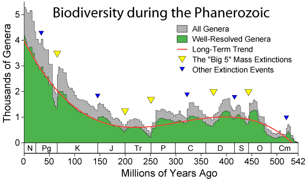
6. Anthropocene: Debated start, from 15,000 years ago to 1950- present

• • Humans have caused 75% of extinctions since the 1600s

Drivers of Biodiversity:

• Age of Community
• Climate Stability
• Energy Availability: evapotranspiration can be used as a proxy for photosynthesis at the base of the food chain
  • Increasing plant energy available = increasing animal diversity  
• Spatial Heterogeneity
  • Habitat heterogeneity increases the number of species (alpha diversity) and variation between communities (beta diversity)
• Ecosystem Productivity
  • Net primary productivity by plants increases overall ecosystem productivity
  • When environmental conditions are favorable for photosynthesis, many tree species can be supported which leads to greater plant diversity over time and creates niche space for greater animal diversity
• Land Area
• Migration: can cause diversity to vary seasonally

Biodiversity Patterns:

• Patterns in North America:
  • Endemic species are concentrated in the Southeast
  • Mammals have more biodiversity in the West and North than the Southeast
  • Diversity is highest near water sources, specifically around the Mississippi River
• Global Patterns:
  • Biodiversity increases near the equator
  • Amphibian diversity is highest in South America and lowest in desert areas
  • Bird diversity is highest in tropical areas
  • Marine environments have high numbers of threatened species worldwide, and Brazil and the US have high numbers of threatened bird species
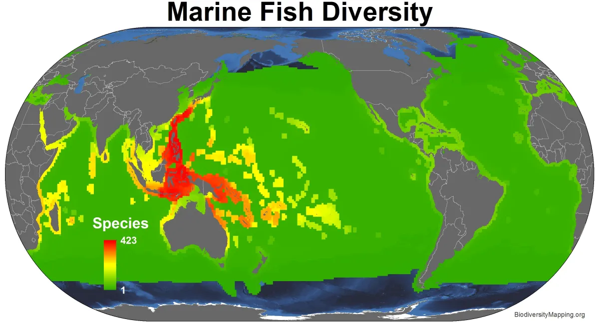
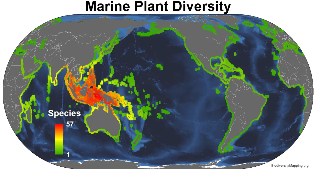
  • Marine biodiversity is greatest in the Pacific, near Southeast Asia and Australia
• Species Diversity Distributions 
  • Terrestrial diversity increases as you near the equator (latitudinal gradient) and decreases in deserts
    • “Equatorial peaks” and “Desert drops”
    • Most species follow this pattern
      •  Exceptions: species whose diversity follows the opposite or whose diversity is more closely correlated with longitudinal gradients

Blog Style Summary:

When someone asks you “What does biodiversity mean to you?” many definitions may come to mind. Probably the simplest definition of biodiversity is: the variety and variability of life on Earth. Now, just how much biodiversity is there on our planet? In 2008 there were 1.6 million known species, in 2009 there were 1.9 million, and in 2015 there were 2,391,916. Currently, there are 2,392,042 known species. However, there are estimated to be 8.7 million eukaryotic species and up to 1.6 million prokaryotic species in total. This means that a majority of life on Earth has yet to be found or classified!

The Earth hasn’t always been like this, however. There have been 5 mass extinction events, or events in which over 75% of species have gone extinct within a 2 million year period since life began on this planet. However, mass extinctions don’t spell total doom for biodiversity. Exponential growth in species has occurred before some, and after all, mass extinction events. This illustrates that while mass extinction events do imply doom for many, they also open up niches for other species to thrive and evolve. For example, we wouldn’t have those cute and fluffy mammals we all love if dinosaurs hadn’t gone extinct!

You may be wondering how the amount of species we have on Earth is determined in the first place. Biodiversity can be estimated through multiple methods: rarefaction, fossil records, and DNA sequencing. Chao1 is a method used to estimate the richness of species within a population based on a sample from the community. Rarefaction is another method used to assess species richness from the results of sampling. Figure 1 below shows a rarefaction curve. Section A of the curve shows that new species are being found with every sample taken, section B shows that there are some repeat species found with each sample but there are still new ones being found, and section C shows that you are only finding repeat species so all of them have most likely been found. Rarefaction curves can be used to gauge how much sampling is “enough” to get an accurate picture of the species composition of the community.

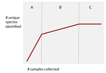
Figure 3. Rarefaction curve from Quiz #5 on Moodle

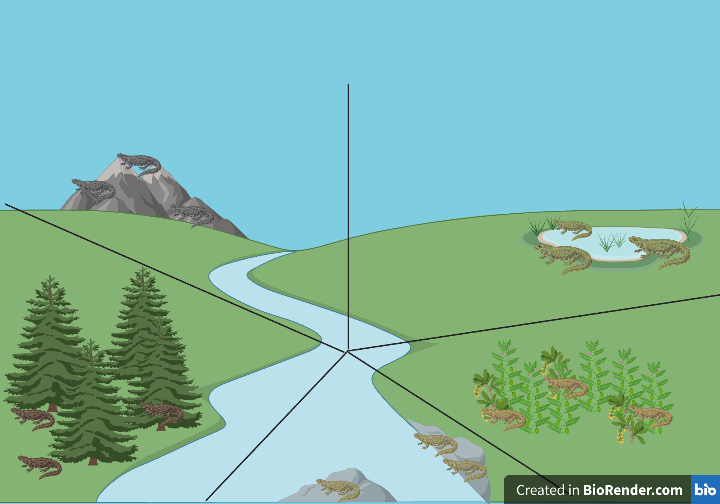
Ever wonder why a red maple tree isn’t found in the desert or why moose don’t live in North Carolina? It is because environmental patterns such as water availability, temperature, climate, geology, habitat connectedness, and the age of a community, are highly variable across geographic regions. A desert is too arid for a red maple tree and North Carolina is too hot for moose. These differences in environmental conditions lead to higher global biodiversity because no one species can be perfectly adapted for this wide range of conditions. Other conditions, such as energy availability and ecosystem productivity, also influence species diversity. Land areas with conditions ideal for plant photosynthesis- ample sunlight, frequent rainfall, and moderate temperatures- support plant growth. In turn, high plant growth and high plant diversity are able to support more diverse fauna. The same can be said about marine environments. Shallow water areas receive more sunlight and nutrients from upwellings that in turn support more plant growth. More plant growth supports a higher diversity of fish (Figure 2).

When looking at various maps of diversity across the globe, we notice some similar trends and patterns. One noticeable trend is that diversity is often highest towards the equator (sometimes called an equatorial peak). This is likely due to a larger input of energy (sunlight) allowing for greater plant productivity, which benefits higher trophic levels.
Rainforests provide a dramatic example of biodiversity in tropical and subtropical areas. On the opposite end of the spectrum, biodiversity decreases in desert regions; this is known as a diversity dip. The harsh climate and geography of desert regions do not allow many species to survive.

Understanding species diversity patterns will be important as climate change alters environmental conditions and shifts habitat ranges. Changes in biodiversity can be a symptom of change in ecology, health, climate, or other biotic and abiotic factors. Climate change, habitat loss, and other anthropogenic factors have all contributed to a declining global biodiversity. Understanding how and why species exist where they do, and how environmental changes are impacting them, will help us better conserve the remaining biodiversity we have left.

Spotlight on NC:

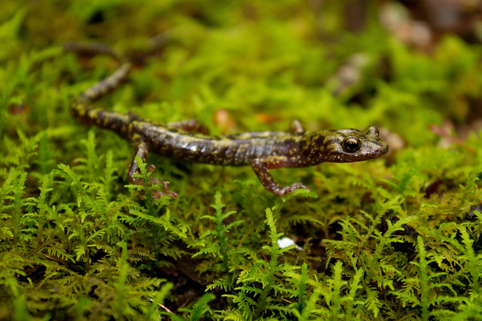
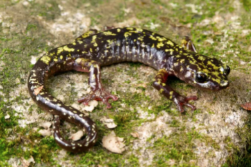
Green Salamander: A Lesson in Biodiversity

One fact that always amazes me is that 99% of life that has lived on this planet has gone extinct. As big and vast as all the current life on Earth seems, it is only a tiny fraction of all the different kinds of life that have ever existed. The variety of life that currently exists on Earth is referred to as biodiversity. This word is probably giving you déjà vu as it is constantly being thrown around in the news, specifically in stories about how humans are causing global declines in biodiversity. As you can probably guess, declining biodiversity is a very bad thing. Declines in biodiversity mean ecosystems are less productive, less healthy, and more unstable. This leads to cascading effects across trophic levels and on the global scale.

While we are usually guilty of only thinking about biodiversity in terms of our favorite zoo animals, there are almost 2.4 million species of all kinds of life out there. While this may seem intimidating, much of this number are microscopic forms of life, which are still very important to all other walks of life. In this blog post, we’ll be taking a deep dive into a tiny little species in North Carolina that shows the ginormous concept of biodiversity and why it is so important.

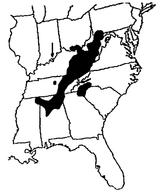
Deep in the Appalachian mountains, at the junction between North Carolina, Georgia, and South Carolina, you may be lucky enough to find the Green salamander (Aneides aeneus) [Fig 1.]. They belong to the Plethodontidae family of lungless salamanders. The Green salamander is somewhat unique among other Aneides species however, as it and only one other species, the Hickory Nut Gorge green salamander, are found along the Eastern portion of the United States [1]. This species prefers to spend the majority of its time inside moist rocky crevices within the mountains, which provide them with protection while keeping them moist so they can breathe through their skin [2]. A 2005 study found that arboreal or woody spaces, namely those with hardwood trees, also provide important habitat for these salamanders. While their damp, rocky outcrops keep them safe during the colder winter months, when spring comes the salamanders migrate towards nearby trees and the surrounding leaf litter and remain primarily arboreal throughout summer [3].

Ranging from about 8-12 cm long, the Green salamander is a medium-sized member of its family, with square-tipped toes that aid them in climbing. This enhanced ability to climb allows them to be excellent insectivores, feeding on spiders, ants, mites, and other arthropods [4]. Despite their excellent hunting abilities, the Green salamander still faces predation risks of its own- mostly from snakes and spiders, which are able to fit into the same rock crevices the salamanders call home. Predatory attacks such as these aren’t exclusive to adult salamanders- they threaten their eggs as well. Unlike most other salamander species, Green salamanders undergo direct development in the egg, hatching as a “mini” adult. This differs from most other amphibians as their eggs do not need to be laid in a water source, and their young skip the typical aquatic larval stage that most salamander species experience [5]. This strategy for reproduction only further highlights the need for these damp rock crevices, as their role in keeping the eggs moist is crucial for offspring survival.

Green salamanders in particular have faced a lot of challenges over the last few decades. Population estimates from across their ranges have shown a decline of up to 98% in some areas, compared to their 1970 populations [6]. The causes of their decline are likely a combination of habitat fragmentation, overcollection by scientists, climate change, and, to a degree, outbreaks of chytrid fungus – a deadly fungus that has been decimating amphibian populations globally. Climate change, namely adverse weather conditions here, seems to be a major cause of the decline of this species. Temperature-related mortality was proposed as the likeliest cause for the die-offs of these salamanders, and the overlap between the winter of 1996-1997 and a large proportion of salamander deaths points to this. All of these working together against the Green salamander have led to an IUCN listing as “near threatened”, along with varying local classifications, such as Indiana’s “state endangered” listing [7].

Hickory Nut Gorge Salamander

Deep within the Smoky Mountains lies 12 million years worth of evolution and one impressive biodiversity hotspot in North Carolina [8]. Hickory Nut Gorge is what some have phrased, “an ecological treasure” and is home to 37 rare plant species and 14 rare animal species [9]. Ecosystem productivity is particularly high in this area of sheer granite cliffs and undisturbed forest. The diversity of salamanders in North Carolina is expansive, with 64 species found statewide, however, Hickory Gorge hides a small, green emerald that has isolated itself within the rocky crags [8].

After fighting off the sheer panic of 14 miles worth of steep cliffs and tumultuous water, one may be lucky enough to spot the Hickory Nut Gorge green salamander (Aneides caryaensis) [Fig. 3]. Discovered in 2019 by an eager scientist named J.J. Apodaca, its bright green spots, adhesive toe pads, and long arms make it suited for the rugged terrain [10]. The Hickory Nut Gorge green salamander (phew quite a long name for such a little guy!) can breathe without lungs and is endemic to the gorge [8]. While its name may insinuate that it’s just another green salamander, due to environmental heterogeneity it is actually a genetically distinct species [8]. Unfortunately, its small ecosystem range and specialization that gave it its name makes it particularly vulnerable to climate change, anthropogenic effects, disturbances, and inbreeding, leading it to have an IUCN classification of “critically endangered”[11, IUCN]. Petitions have been formed in an effort to provide federal protections for the Hickory Nut Gorge green salamander under the Endangered Species Act. Hopefully, this will help mitigate its rapid decline and prevent its extinction [11].

You may be wondering why it’s so important to conserve this small, endangered species, after all, it lives in one of the most isolated parts of the Smoky Mountains. Well, the Hickory Nut Gorge green salamander plays a key role in ecosystem biodiversity and food web interactions [11]. It assists in nutrient cycling, reduces pests, and links invertebrates and vertebrates together [11 & 10]. Without this salamander, interspecific interactions may decline and the biodiversity of the Smoky Mountains may suffer. Though the Hickory Nut Gorge green salamander is only one species in a region of expansive biodiversity, it is a crucial key in protecting the livelihood of its natural habitat.

Featured Ecologists:

Sylvia Earle, Phd

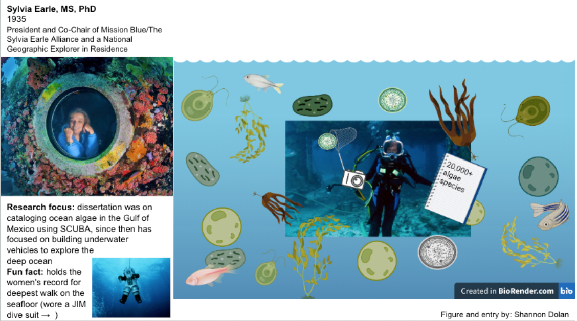
Sylvia Earle revolutionized marine ecology and biology research. She cataloged over 20,000 species of algae and aquatic plants in the Gulf of Mexico using SCUBA. SCUBA was a new technology, so her research was some of the first research studies to use SCUBA. Her research question was what type and distribution of algae are present; her findings provided a vast amount of insight into the ocean landscape. This connects to the concepts of biodiversity and species distribution patterns we’ve discussed in class. Earle has become a major advocate for ocean conservation.

In the 1970s, she also was the lead scientist on the Tektite II Project, which involved scientists living and conducting research 50 feet underwater. (Side note: The government did not want a male and female crew–and would have preferred a male-only crew–but Sylvia Earle was the most experienced diver. So instead, Earle led an all-women team to live and collect photographs of marine life 50 feet underwater for two weeks.) The crew photographed and studied the effects of pollution on coral. In her mid-career, she gave talks around the world about her deep-sea explorations and helped ignite a passion in others for conserving marine life. Dr. Earle eventually became the first woman to be the Chief Scientist of the National Oceanic and Atmospheric Administration (NOAA). She was also named the first Time magazine “Hero of the Planet”. In total, she has spent over 7,000 hours underwater and has authored over 200 papers.

Rosemary Gillespie, Phd

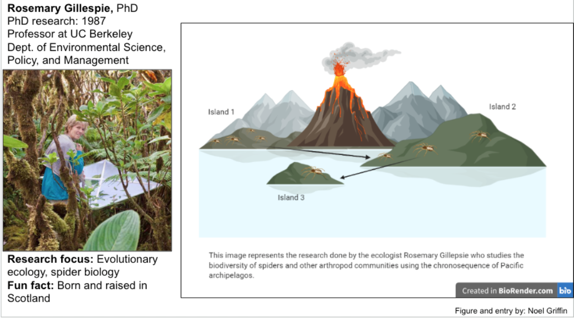
Rosemary Gillespie mainly researches the evolutionary patterns of arthropods on the Pacific islands or archipelagos. Some of her research has included using metabarcoding and machine learning of arthropods, and analyzing arthropod species and population assemblage based on the Hawaii islands’ chronosequence. Gillespie’s research relates to our class material because she is interested in better understanding the drivers of the biological diversity of populations such as geography, invasive species, migration, and trophic levels. Gillespie’s major findings are discovering the various impacts of global change on the biodiversity of arthropod communities. The research performed by Gillespie is important because it broadens our knowledge of how biodiversity changes over time as a result of global change. Arthropod communities are the most diverse macrobiota on Earth and play critical roles in food webs so understanding the changes in their biodiversity is needed. Gillespie supports others to pursue science careers also. She has led many programs that encourage undergraduates to participate in biological research.

Ruth Patrick, Phd

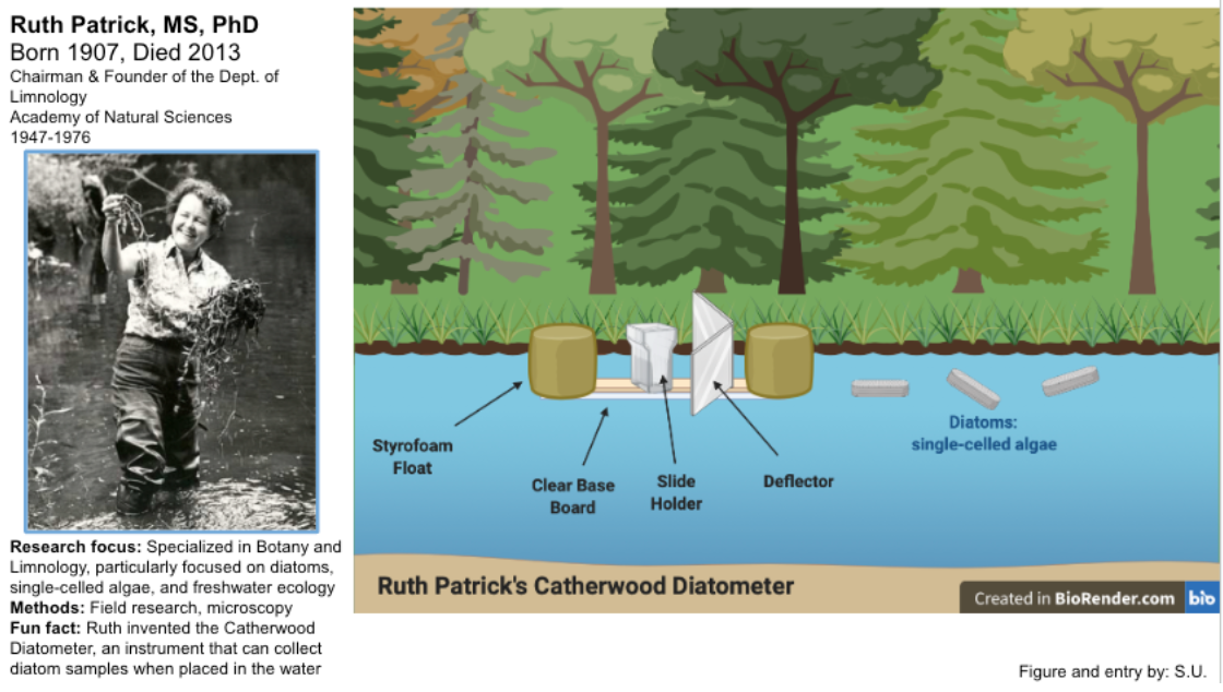
Dr. Ruth Patrick was one of the pioneers in studying diatom biodiversity as a way to understand the health of a body of freshwater. She also specialized in understanding the effects of pollution on the health of rivers, lakes, and drinking-water sources by studying diatom response. In 1945, she invented the Catherwood diatometer, an instrument that can collect diatoms, a group of single-celled algae, and was the first to claim that a healthy diatom composition in a body of freshwater should be species-rich and diverse. She then used this to prove that pollution had an effect on diatom composition. She was also the first to identify the health of a river based on plant and animal composition alone, giving rise to what’s known as the Patrick Principle: the belief that biodiversity is the chief indicator of water health. Her research of fossilized diatoms found that the Great Dismal Swamp between North Carolina and Virginia was once a forest, and also that the Great Salt Lake was not always salty. Her research on the health of streams and rivers by monitoring diatom diversity sparked national interest and research in diatom science, not to mention that after volunteering and working for the Academy of Natural Sciences for many years, she became the first woman and the first environmentalist to serve on the DuPont board of directors in the 1950s. She went on to consult Presidents Lyndon B. Johnson and Ronald Reagan on water quality issues such as pollution and acid rain, and earned the National Medal of Science from Bill Clinton in 1966.

Student contributors:

Note Outline: Paige Fryar, Brooke Burns, Evelyn Rowan, Jakob Fix

Blog Style Summary: Iris Horton, Shannon Dolan, Hannah Werner, Tessa Ferguson

Spotlight on NC: Eli Benbenek, Rebecca Olson, Trey Kaufman

Featured Ecologists: Shannon Dolan, Noel Griffin, S.U.