5 Pace of Evolution

By the end of this chapter, you wil be able to do the following:

• Describe the two parts of a gene: introns and exons
• Explain the role that exons play in evolution
• Explain the two major theories on rates of evolution
• Compare and contrast adaptation theory to neutral theory
• Describe how the molecular clock is used by scientists
• Apply the molecular clock to determine evolution rates

Introduction

Evolution can occur through various means: adaptive natural selection and non-adaptive genetic drift, gene flow, and mutations.  How quickly can such change occur?   Darwin envisioned changes occurring so slowly that we would never be able to see evidence of evolution in our lifetime.  We know this is not true.  For example, bacteria and pathogens can respond quickly to a toxin or antibiotic and we have evidence natural selection can occur rapidly.  But what about larger organisms, such as animals?  Can they undergo evolution quickly?  And do some types of evolution occur more rapidly than other types?

As we have discussed in previous chapters, genetic drift occurs more quickly with smaller populations compared to large populations.  The pace of evolution, regardless of which mechanism is in play, does occur more quickly as the population size decreases. But there is more at play than just population size.  What about which type of DNA is subject to evolutionary change?  What about how DNA changes over time – does it always change for the better, the worse, or change nature (like move from something functional to something non-functional)?  Let’s explore these topics in more detail.

Introns and Exons

Before moving forward, it will be helpful to get a context of DNA and genes more fully.  As you know, DNA is a double-stranded molecule made up of sugars, phosphates, and bases.  These bases are arranged in a specific order that dictates the types of proteins that are made.  The DNA is copied into a mRNA strand (in a process called transcription) so that is can be translated into a protein.  A message of three bases, called a codon, provides the instructions for an amino acid (the building block of a protein).  For example, the codon AGC (adenine-guanine-cytosine) is a message for the amino acid serine.  You can see other examples of the genetic code below (Fig 1).

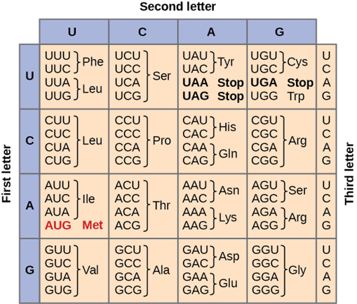
Figure 1: The genetic code for translating each nucleotide triplet into an amino acid of a protein.  From https://courses.lumenlearning.com/suny-osbiology2e/chapter/the-genetic-code/ 

When we examine the DNA sequencing or the mRNA sequencing, we find on average that a typical gene, or a message for a trait, contains about 2000 nucleotides.  Not all of these nucleotides will code for amino acids.  In fact, some of them will be cut out of the mRNA strand and degraded.  These discarded sections of mRNA tend to be repetitive in nature and are called introns.  They will not code for proteins.

The sections of DNA and corresponding mRNA that do provide the message for proteins are called exons.  These sections of genetic material are therefore important for providing those instructions for making proteins in the body.

Consider how DNA mutations can be different depending on the location of where that mutation occurs.  If a mutation occurs in an intron, there may not be any effect.  The introns are not actively coding for a protein or a trait.  If, however, a mutation occurs in the exon of DNA, there may be a problem.  If the mutation is a silent mutation or a non-point mutation, the amino acid and protein will not be affected.  For example, if our AGC codon, which codes for serine, changes to AGU, serine is still going to be made (Fig 1).  This is because of the redundancy of the genetic code – there is more than one codon that give the instructions for making that one amino acid.

If a point mutation occurs in an exon, things can be different.  If that AGC codon has a change such that it is now CGC, we now have a different amino acid, arginine.  This is a new amino acid and as such you will see a new protein being made.  If this new protein or trait is beneficial to the cell and organism, you might expect natural selection to favor it and for the new trait to become more prevalent in the subsequent generations.  If the new trait occurs in a small population, you might expect genetic drift to occur and for it to change again or for it to increase in frequency.

Gradualism and Punctuated Equilibrium and their connection with Microevolution and Macroevolution

When people consider evolutionary change, we are typically talking about exons and traits changing so that we physically see something different.  Maybe it is a different fur color that we see in a population of rabbits or maybe a different beak length in a population of birds.

When Darwin was considering evolutionary change, he was thinking about changes with what the population already had – seeing a frequency change between one variation of the trait to another variation (depending on the selective pressure).  This type of change was indicative of microevolution.  You could see a change within the species itself as the population was adapting to the environment.

If a change occurred such that a new species was carved out, we use the term macroevolution.  Here, you might find many traits changing over time, building up to cause enough changes that we no longer recognize that ancestor species and determine that a new species is being formed or has formed.

Darwin believed that gradual changes accumulated over evolutionary time to slowly result in macroevolution.  He believed that we would see evidence of this in the fossil record with an ancestor species evident, transitional species shown, and the modern species exhibited.  This is often referred to as phyletic gradualism (Fig 2).  Again, with gradualism, you see over evolutionary time, small gradual changes that will eventually diverge into new species.  You would find intermediate and transitional species over evolutionary time.

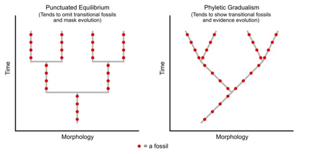
Figure 2: Fossils in punctuated equilibrium versus fossils in phyletic gradualism.  Notice on the left that the species will stay in equilibrium, without change, for a long time (this is shown with a straight vertical line), before it rapidly changes course with speciation (shown as the football goal post).  With gradualism on the right, notice there are no vertical non-changing lines.  Instead, there is constant, but slight, change, leading to speciation events.  Faus, CC , via Wikimedia Common

A common illustration of this is with horse evolution.  We see in the fossil record gradual changes from 4-toed, fox-sized creatures 50 million years ago to today’s larger 1-toed horse.  We also see changes in the teeth over time, gradually transforming the size and structure of dentition and individual teeth due to the selective pressures of changing diet and predation.  Individuals with longer limbs could live longer and reproduce more because they could evade predators.  And individuals with larger, more grinding teeth, could obtain more energy from the grazing lifestyle and live longer and reproduce more, passing on this trait (Fig 3).

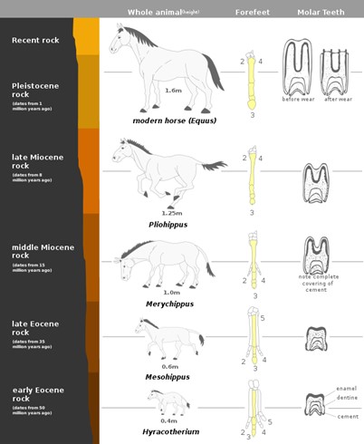
Figure 3: The evolution of the horse.  Notice that the number of toes has been reduced over time as well as the tooth structure.  Original:  Mcy jerry Vector:  SarangPixelsquid, CC, via Wikimedia Commons 

Another idea for carving out new species is found with punctuated equilibrium.  Punctuated equilibrium derives its name from the fact that in fossil record you can see no change (equilibrium) for a long time.  The species is static without change.  Then, in the fossil record, you quickly see that punctuated change and very quickly a new species appears.  There is no transitional or intermediate species (Fig 2).  This rapid change is geological time, so we are talking about perhaps fewer than 100,000 years for significant change.  The rapid changes are thought to occur in response to this sudden environmental changes or other factors and as such, you would be more likely to see punctuated equilibrium change occurring in a small population. Punctuated equilibrium always addresses macroevolution.  While punctuated equilibrium suggests a faster tempo, it does not necessarily exclude gradualism (Fig 4).

Again, the primary influencing factor on changes in speciation rate is environmental conditions. Under some conditions, selection occurs quickly or radically. Consider a species of snails that had been living with the same basic form for many thousands of years. Layers of their fossils would appear similar for a long time. When a change in the environment takes place—such as a drop in the water level—a small number of organisms are separated from the rest in a brief period of time, essentially forming one large and one tiny population. The tiny population faces new environmental conditions. Because its gene pool quickly became so small, any variation that surfaces and that aids in surviving the new conditions becomes the predominant form.

Punctuated equilibrium can work in concert with gradualism and natural selection.  They are not necessarily mutually exclusive.  Punctuated equilibrium predicts rapid evolutionary change leading to new species forming in a short geological time period.  After such a rapid change, you might then expect natural selection and possibly gradualism to lead to further changes.

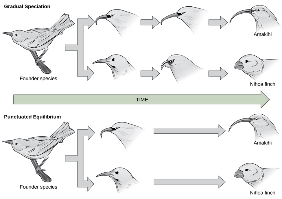
Figure 4: In (a) gradual speciation, species diverge at a slow, steady pace as traits change incrementally. In (b) punctuated equilibrium, species diverge quickly and then remain unchanged for long periods of time.

Adaptive Theory and Neutral Theory

Darwin’s ideas of bouncing between genotypes with the highest fitness given the selective pressure works well when considering how the environment might change over time.  If the environment is continually changing, there will not be one allele that becomes “fixed” in the population.  This means that at any given time, one allele might be more adaptive compared to the other, but that it is relative.  If the environment changes, and the selective pressure changes, that same allele may no longer be the most adaptive.  Recall that “adaptive” refers to traits or characteristics of an organism that confer a selective advantage, increasing its chances of survival and reproduction within a specific environment, compared to peers in the population. These adaptive traits are better suited to the ecological conditions and challenges faced by the organism, allowing it to effectively compete for resources, evade predators, and successfully reproduce.

What is being described above is essentially what we now call the Adaptive Selection Theory (or Adaptive Theory).  As indicated by the name of this theory, it centers around natural selection.

An alternative to this is the Neutral Theory.  Here we will see elements of chance being brought in.  The Neutral Theory states there is a balance between mutation and genetic drift that is responsible for maintaining the diversity of alleles and DNA changes that we see over time.  The full name of this theory is the Neutral Theory of Molecular Evolution, which calls attention to the DNA and the idea that an allele is selectively neutral if natural selection is taken out.  That is natural selection does not favor the allele.

We find that introns will come into play often with the Neutral Theory.  For example, if a mutation occurs in an intron, it will not matter since these sections of DNA do not code for proteins or traits.  Dr. Kimura who proposed the Neutral Theory in 1968 calls out that all the variation we see in chromosomes is selectively neutral with most of the changes at the DNA being selectively neutral as well.

If the DNA sequence does change over time, some process other than selection is responsible.  The primary driver in this case is genetic drift.  The variation of the alleles and all the genetic diversity at a particular place on a chromosome is present because all the variations work.  They are all equally good at their jobs so to speak and in that sense the variation is neutral.  A movement from one version to another occurs due to genetic drifting.

Molecular Clock

When scientists look at evolutionary changes over long periods of time, they can see patterns and trends.  The rates of molecular evolution are constant over time, like seconds in a clock – predictable and constant.  This is where the term molecular clock comes from.  It is the neutral theory in action, explaining how the constancy of rates could be.  This concept was first put forward in 1962 by chemist Linus Pauling and biologist Emile Zuckerkandl and was based on the observation that genetic mutations occur at a relatively constant rate.

When we have a large sample size (again, looking at molecular data over evolutionary time) we find a constant change occurring in the DNA sequences that is occurring too quickly and too consistently to be explained by natural selection.  Instead, if we consider neutral changes, those caused by genetic drift and in introns or neutral alleles, it is predicted these become constant and consistent over evolutionary time.  That is, over the course of millions of years, neutral mutations will build up in any given stretch of DNA at a reliable rate – this is the molecular clock.

This predictable rate then becomes a power tool for estimating when speciation occurred or when major traits evolved.  For example, if you know the rate of change for species, you can use that information to calculate the time of their last ancestor (Fig 5).  You can also use information known to determine the rate of evolution in different ways.  For example, if you know the mutation rate of a gene and are trying to understand how much genetic difference there is between two species, you can use the date of the last common ancestor to determine this answer using the following formula:

Genetic Difference – Mutation Rate X Time

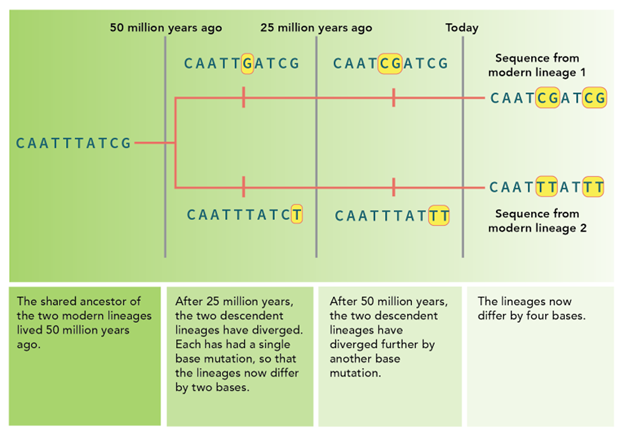
Figure 5: If we compare two species (lineage 1 on top to lineage 2 on the bottom) we can see these species differ by four bases (highlighted).  If we know that this entire length of DNA changes at a rate of approximately one base per 25 million years, that means that the two DNA versions differ by 100 million years of evolution and that their common ancestor lived 50 million years ago.  From https://evolution.berkeley.edu/molecular-clocks/

The molecular clock is measuring the number of changes or mutations that accumulate over time.  The more changes you see between two species, the less related they are and the more distant their last common ancestor.  Scientists are using the number of mutations in a given stretch of DNA to measure time.

It is worth noting that some genes or stretches of DNA, evolve at different rates.  Recall that conserved genes, typically associated with vital proteins, change very slowly if at all over evolutionary time.  Genes associated with less vital functions and neutral alleles occurs more rapidly.  Scientists have solved this issue by taking the known amounts of genetic change and calibrating it against known amounts of elapsed time.  This is called fossil calibration.  If we have a fossil of the ancestor we can use radiometic dating and tell how long ago it lived and this will be used to help determine the molecular clock rates.

Because scientists can use molecular clock data in the absence of fossils, we have been able to determine many events.  Since the molecular clock can use the constant rate that is calculates for a group of species, the genetic difference between any two species is proportional to the time since these species last shared a common ancestor.  For example, the molecular clock has been used to estimate that the conserved cytochrome b genes in birds evolve at an average rate of approximately 1% per 1 million years (Weir & Schluter 2008).  This means that any two bird species are diverging from each other at a rate of 2% per 1 million years and has been regarded as the “2% rule” and used widely by scientists.

The molecular clock can also be used to help determine the impacts of climate events on speciation, geological events on speciation, date the origin of gene families, determine the timing of dispersal events, and identify novel trait timing events.  It can also be used in a more modern-day application to study disease events.  For example, in 2012 researchers determined that India’s HIV-1 subtypes had a common ancestor 40 years prior and they used those data to infer the spread of the virus to inform medical policy, predicting where HIV would spread and therefore utilize resources, such as educational campaigns, to help save lives (Neogi et al 2012).

Summary

The concept of the molecular clock contributes to our understanding of evolutionary relationships and species divergence by providing a mechanism for natural selection and the Neutral Theory, while explaining the process of genetic drift.  The molecular clock can also be used to estimate the rate of genetic mutations over time as well as being put to use in a predictive way to help with policy decisions.

The neutral theory of molecular evolution suggests that the majority of genetic mutations that occur at the molecular level are selectively neutral, meaning they neither provide a significant advantage nor a disadvantage to an organism’s survival or reproduction. These neutral mutations are thought to accumulate in populations over time through genetic drift.

The neutral theory is applied to explain patterns of genetic diversity within populations by proposing that much of the observed genetic variation is the result of neutral mutations spreading through populations due to chance rather than natural selection. This theory helps us understand how genetic diversity can persist and accumulate even in the absence of strong selective pressures.

In essence, the neutral theory highlights the role of random genetic drift as a major factor in shaping the genetic makeup of populations, particularly at the molecular level. It offers an alternative perspective to the traditional emphasis on natural selection as the primary driver of evolution.

Questions

Glossary

References

Clark, MA, Choi, J, and Douglas, M. Biology 2e for Biol 111 and Biol 112.

Kosal, E. 2023. NC State University.

Neogi U., Bontell I, Shet A, De Costa  A, Gupta S, Diwan V, Laishram RS, Wanchu A, Ranga U, Banerjea AC, & A Sonnerborg. 2012. Molecaulr epidemiology of HIV-1 subtypes in India: Origin and evolutionary history of the predominant subtype C. PLoS One 7(6): e39819. doi: 10.1371/journal.pone.0039819

Weir, JT, & D Schluter. 2008. Calibrating the avian molecular clock. Molecular Ecology 17 (10): 2321-2561..  https://doi.org/10.1111/j.1365-294X.2008.03742.x