17 Population Ecology

By the end of this chapter you will be able to:

• Describe how ecologists measure population size and density
• Predict how populations will grow over time by applying population growth equations
• Describe the three types of survivorship curves and relate them to specific populations
• Explain the characteristics of and differences between exponential and logistic growth patterns
• Give examples of how the carrying capacity of a habitat may change
• Compare and contrast density-dependent growth regulation and density-independent growth regulation

Introduction

A population is a group of organisms of the same species interacting in a given area.  Populations are dynamic entities. Their size and composition fluctuate in response to numerous factors, including seasonal and yearly changes in the environment, natural disasters such as forest fires and volcanic eruptions, and competition for resources between and within species. The statistical study of populations is called demography: a set of mathematical tools designed to describe populations and investigate how they change. Many of these tools were actually designed to study human populations; however, while the term “demographics” is sometimes assumed to mean a study of human populations, all living populations can be studied using this approach.

Populations are characterized by their population size (total number of individuals) and their population density (number of individuals per unit area). A population may have a large number of individuals that are distributed densely, or sparsely. There are also populations with small numbers of individuals that may be dense or very sparsely distributed in a local area. Population size can affect the potential for adaptation because it affects the amount of genetic variation present in the population. Density can have effects on interactions within a population such as competition for food and the ability of individuals to find a mate. Smaller organisms tend to be more densely distributed than larger organisms (Fig 1) likely because smaller animals require less food and other resources, so the environment can support more of them per unit area.

Figure 1: Australian mammals show a typical inverse relationship between population density and body size.

Estimating Population Size

The most accurate way to determine population size is to count all of the individuals within the area; however, this method is usually not logistically or economically feasible, especially when studying large areas. Thus, scientists usually study populations by sampling a representative portion of each habitat and use this sample to make inferences about the population as a whole. The methods used to sample populations to determine their size and density are typically tailored to the characteristics of the organism being studied. For immobile organisms such as plants, or for very small and slow-moving organisms, a quadrat may be used. A quadrat is a wood, plastic, or metal square that is randomly located on the ground and used to count the number of individuals that lie within its boundaries (Fig 2). To obtain an accurate count using this method, the square must be placed at random locations within the habitat enough times to produce an accurate estimate. This counting method will provide an estimate of both population size and density. The number and size of quadrat samples depends on the type of organisms and the nature of their distribution.

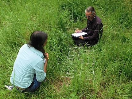
Figure 2: London Wildlife Trust Ecologist Tony Wileman and assistant carrying out a transect survey of the anthill meadow in Gunnersbury Triangle local nature reserve. The quadrats are placed every 2 metres along the transect line and all the plants in the sample areas are listed. Ian Alexander, CC via Wikimedia Commons

For smaller mobile organisms, such as mammals, a technique called mark and recapture is often used. This method involves marking a sample of captured animals in some way and releasing them back into the environment to mix with the rest of the population; then, a new sample is captured and scientists determine how many of the marked animals are in the new sample. This method assumes that the larger the population, the lower the percentage of marked organisms that will be recaptured since they will have mixed with more unmarked individuals. For example, if 80 field mice are captured, marked, and released into the forest, then a second trapping 100 field mice are captured and 20 of them are marked, the population size (N) can be determined using the following equation:

(number marked first catch X total number second catch) / number marked second catch = N

Using our example, the population size would be 400.

(80 × 100) / 20 = 400

These results give us an estimate of 400 total individuals in the original population. The true number usually will be a bit different from this because of chance errors and possible bias caused by the sampling methods.

Scientists can get very creative in how they capture animals to study them.  Watch this video to learn more about how scientists use electricity to study blue catfish populations (which can grow more than 5 feet in length!).

Species Distribution

In addition to measuring density, further information about a population can be obtained by looking at the distribution of the individuals throughout their range. A species distribution pattern is the distribution of individuals within a habitat at a particular point in time—broad categories of patterns are used to describe them.

Individuals within a population can be distributed at random, in groups, or equally spaced apart (more or less). These are known as random, clumped, and uniform distribution patterns, respectively (Fig 3). Different distributions reflect important aspects of the biology of the species; they also affect the mathematical methods required to estimate population sizes. An example of random distribution occurs with dandelion and other plants that have wind-dispersed seeds that germinate wherever they happen to fall in favorable environments. A clumped distribution, may be seen in plants that drop their seeds straight to the ground, such as oak trees; it can also be seen in animals that live in social groups (schools of fish or herds of elephants). Uniform distribution is observed in plants that secrete substances inhibiting the growth of nearby individuals (such as the release of toxic chemicals by sage plants). It is also seen in territorial animal species, such as penguins that maintain a defined territory for nesting. The territorial defensive behaviors of each individual create a regular pattern of distribution of similar-sized territories and individuals within those territories. Thus, the distribution of the individuals within a population provides more information about how they interact with each other than does a simple density measurement. Just as lower density species might have more difficulty finding a mate, solitary species with a random distribution might have a similar difficulty when compared to social species clumped together in groups.

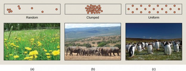
Figure 3: Species may have a random, cluped, or uniform distribution.  Plants such as (a) dandelions with wind-dispersed seeds tend to be randlomly distributed.  Animals such as (b) elephants that travel in groups exhibit a climped distribution.  Territorial birds such as (c) penguins tend to have a uniform distribution. (credit a: modification of work by Rosendahl; credit b: modification of work by Rebecca Wood; credit c: modification of work by Ben Tubby)

Survivorship Curves

Ecologists can also study populations with the use of a survivorship curve, which is a graph of the number of individuals surviving at each age interval versus time. These curves allow us to compare the life histories of different populations (Fig 4). There are three types of survivorship curves. In a type I curve, mortality is low in the early and middle years and occurs mostly in older individuals. Organisms exhibiting a type I survivorship typically produce few offspring and provide good care to the offspring increasing the likelihood of their survival. Humans and most mammals exhibit a type I survivorship curve. In type II curves, mortality is relatively constant throughout the entire life span, and mortality is equally likely to occur at any point in the life span. Many bird populations provide examples of an intermediate or type II survivorship curve. In type III survivorship curves, early ages experience the highest mortality with much lower mortality rates for organisms that make it to advanced years. Type III organisms typically produce large numbers of offspring, but provide very little or no care for them. Trees and marine invertebrates exhibit a type III survivorship curve because very few of these organisms survive their younger years, but those that do make it to an old age are more likely to survive for a relatively long period of time.

Figure 4: Survivorship curves show the distribution of individuals in a population according to age.  Humans and most mammals have a Type I survivorship curve, because death primarily occurs in older years.  Birds have a Type II survivorship curve, as death at any age is equally probably.  Trees have a Type III survivorship curve because very few survive the younger years, but after a certain age, individuals are much more likely to survive. 

K-Selected and r-Selected Species

Ecologists use the terms “K-selected” and “r-selected” to describe a species’ reproductive strategy in relation to the carrying capacity (K) of its environment. This concept was developed by the ecologists Robert MacArthur and E. O. Wilson and is an important aspect of understanding how different species adapt and thrive in their respective environments.

K-selection is also known as density-dependent selection, where the letter “K” represents the carrying capacity of an environment, which is the maximum population size that can be supported sustainably by the available resources in that particular ecosystem.

Characteristics of K-selected species:

1. Reproductive Strategy: K-selected species typically have a reproductive strategy that focuses on quality over quantity. They invest more time and resources into producing fewer offspring but with a higher likelihood of individual survival and successful reproduction.
2. Offspring Care: These species often exhibit extended parental care for their offspring. They invest time and energy in nurturing and protecting their young, increasing their chances of survival and successful growth.
3. Long Lifespan: K-selected species tend to have longer lifespans compared to r-selected species (the opposite of K-selected). Longer lifespans allow them to invest more in their own survival and reproduction over an extended period.
4. Slow Population Growth: Due to their focus on quality offspring and the resources invested in parental care, K-selected species tend to have slower population growth rates, approaching the carrying capacity of their environment more gradually.
5. Large Body Size: Many K-selected species are larger in size, which often allows for increased energy reserves, better chances of survival, and greater competitive abilities within their ecosystem.
6. Adaptation to Stable Environments: K-selected species are typically well-adapted to stable and predictable environments. They have specialized traits that allow them to efficiently utilize the available resources and successfully compete for them.
7. Interspecific Competition: K-selected species often face significant competition from other individuals of the same species (intraspecific competition) and other species (interspecific competition) for limited resources. Their life history traits are well-suited for coping with these challenges.

Examples of K-selected species include large mammals like elephants, whales, and primates, as well as some bird species with extended parental care and low reproductive rates.

An “r-selected species” is another concept from ecology that describes a species’ reproductive strategy in relation to the rate of population growth (r). The concept of r-selection focuses on species that prioritize rapid reproduction and high population growth rates over the quality of individual offspring.

Characteristics of r-selected species:

1. Reproductive Strategy: r-selected species have a reproductive strategy that emphasizes quantity over quality. They produce a large number of offspring in a short period, increasing the chances that at least some of them will survive and reproduce.
2. Offspring Care: These species often exhibit little or no parental care for their offspring. Once the offspring are born or hatched, they are usually left to fend for themselves. This lack of parental investment allows the species to allocate more energy towards producing more offspring.
3. Short Lifespan: r-selected species tend to have shorter lifespans compared to K-selected species. Their focus on rapid reproduction and population growth means that individual survival and longevity are not as critical to the species’ success.
4. Rapid Population Growth: Due to their high reproductive rates and minimal parental care, r-selected species can experience rapid population growth, often exceeding the carrying capacity of their environment. However, this growth is not sustainable in the long term, and populations may experience boom-and-bust cycles.
5. Small Body Size: Many r-selected species are smaller in size. This can make them more efficient at reproducing quickly and utilizing resources in rapidly changing or unpredictable environments.
6. Adaptation to Unstable Environments: r-selected species are often well-adapted to unpredictable or unstable environments. They are opportunistic and can take advantage of favorable conditions when they arise, even if they are short-lived.
7. Little Interspecific Competition: r-selected species may face less competition from other individuals of the same species (intraspecific competition) and other species (interspecific competition) for resources due to their rapid reproduction and dispersion.

Examples of r-selected species include many insects, small rodents, certain species of fish, and some plants that produce a large number of seeds.

The distinction between r-selected and K-selected species is a general framework and it is often not as clear-cut and straight-forward as ecologists would like it to be.  For example, many species exhibit a mix of characteristics and traits from both strategies depending on their ecological niche and environmental conditions. Additionally, environmental changes can influence a species’ reproductive strategy over time.

Population Growth

Populations grow and change over time.  Often, ecologists want to understand these patterns and they want to be able to make predictions over time.  Consider a conservation manager who is trying to understand a population of an endangered species.  There could also be an application for a game warden who is trying to determine how many individuals of a fish species might be caught in a season.

The two simplest models of population growth use deterministic equations (equations that do not account for random events) to describe the rate of change in the size of a population over time. The first of these models, exponential growth, describes theoretical populations that increase in numbers without any limits to their growth. The second model, logistic growth, introduces limits to reproductive growth that become more intense as the population size increases. Neither model adequately describes natural populations, but they provide points of comparison.

Exponential Growth

Charles Darwin, in developing his theory of natural selection, was influenced by the English clergyman Thomas Malthus. Malthus published his book in 1798 stating that populations with abundant natural resources grow very rapidly; however, they limit further growth by depleting their resources. The early pattern of accelerating population size is called exponential growth.

The best example of exponential growth in organisms is seen in bacteria. Bacteria are prokaryotes that reproduce largely by binary fission. This division takes about an hour for many bacterial species. If 1000 bacteria are placed in a large flask with an abundant supply of nutrients (so the nutrients will not become quickly depleted), the number of bacteria will have doubled from 1000 to 2000 after just an hour. In another hour, each of the 2000 bacteria will divide, producing 4000 bacteria. After the third hour, there should be 8000 bacteria in the flask. The important concept of exponential growth is that the growth rate—the number of organisms added in each reproductive generation—is itself increasing; that is, the population size is increasing at a greater and greater rate. After 24 of these cycles, the population would have increased from 1000 to more than 16 billion bacteria. When the population size, N, is plotted over time, a J-shaped growth curve is produced (Fig 5a).

The bacteria-in-a-flask example is not truly representative of the real world where resources are usually limited; however, when a species is introduced into a new habitat that it finds suitable, it may show exponential growth for a while. In the case of the bacteria in the flask, some bacteria will die during the experiment and thus not reproduce; therefore, the growth rate is lowered from a maximal rate in which there is no mortality. The intrinsic growth rate of a population, r,  is largely determined by subtracting the death rate, D, (number organisms that die during an interval) from the birth rate, B, (number organisms that are born during an interval). The growth rate can be expressed in a simple equation that combines the birth and death rates into a single factor: r, the intrinsic growth rate of a population. This is shown in the following formula:

Population growth (dN/dt) = rN

The value of r can be positive, meaning the population is increasing in size (the rate of change is positive); or negative, meaning the population is decreasing in size; or zero, in which case the population size is unchanging, a condition known as zero population growth.

Figure 5: When resources are unlimited, populations exhibit (a) exponential growth, shown in a J-shaped curve.  When resources are limited, pouplaitons exhibit (b) logistic growth.  In logistic growth, population expansion decreases as resources become scared, and it levels off when the carrying capacity of hte environment is reached.  The logistic growth curve is S-shaped.

Logistic Growth

Extended exponential growth is possible only when infinite natural resources are available; this is not the case in the real world. Charles Darwin recognized this fact in his description of the “struggle for existence,” which states that individuals will compete (with members of their own or other species) for limited resources. The successful ones are more likely to survive and pass on the traits that made them successful to the next generation at a greater rate (natural selection). To model the reality of limited resources, population ecologists developed the logistic growth model.

In the real world, with its limited resources, exponential growth cannot continue indefinitely. Exponential growth may occur in environments where there are few individuals and plentiful resources, but when the number of individuals gets large enough, resources will be depleted and the growth rate will slow down. Eventually, the growth rate will plateau or level off (Fig 5b). This population size, which is determined by the maximum population size that a particular environment can sustain, is called the carrying capacity, or K. In real populations, a growing population often overshoots its carrying capacity, and the death rate increases beyond the birth rate causing the population size to decline back to the carrying capacity or below it. Most populations usually fluctuate around the carrying capacity in an undulating fashion rather than existing right at it.

The formula used to calculate logistic growth adds the carrying capacity as a moderating force in the growth rate. The expression “K – N” is equal to the number of individuals that may be added to a population at a given time, and “K – N” divided by “K” is the fraction of the carrying capacity available for further growth. Thus, the exponential growth model is restricted by this factor to generate the logistic growth equation:

Population growth (dN/dt) = rN X [ (K-N) / K]

Notice that when N is almost zero the quantity in brackets is almost equal to 1 (or K/K) and growth is close to exponential. When the population size is equal to the carrying capacity, or N = K, the quantity in brackets is equal to zero and growth is equal to zero. A graph of this equation (logistic growth) yields the S-shaped curve (Fig 5b). It is a more realistic model of population growth than exponential growth. There are three different sections to an S-shaped curve. Initially, growth is exponential because there are few individuals and ample resources available. Then, as resources begin to become limited, the growth rate decreases. Finally, the growth rate levels off at the carrying capacity of the environment, with little change in population number over time.

The logistic model assumes that every individual within a population will have equal access to resources and, thus, an equal chance for survival. For plants, the amount of water, sunlight, nutrients, and space to grow are the important resources, whereas in animals, important resources include food, water, shelter, nesting space, and mates.

In the real world, phenotypic variation among individuals within a population means that some individuals will be better adapted to their environment than others. The resulting competition for resources among population members of the same species is termed intraspecific competition. Intraspecific competition may not affect populations that are well below their carrying capacity, as resources are plentiful and all individuals can obtain what they need. However, as population size increases, this competition intensifies. In addition, the accumulation of waste products can reduce carrying capacity in an environment.

There are many examples of populations exhibiting logistic growth.  Yeast, a microscopic fungus used to make bread and alcoholic beverages, exhibits the classical S-shaped curve when grown in a test tube (Fig 6a). Its growth levels off as the population depletes the nutrients that are necessary for its growth. In the real world, however, there are variations to this idealized curve. Examples in wild populations include sheep and harbor seals (Fig 6b). In both examples, the population size exceeds the carrying capacity for short periods of time and then falls below the carrying capacity afterwards. This fluctuation in population size continues to occur as the population oscillates around its carrying capacity. Still, even with this oscillation, the logistic model is confirmed.

Figure 6: (a) yeast grown in ideal conditions in a test tube shows a classical S-shaped logistic growth curve, whereas (b) a natgural population of seals shows real-world fluctation.  The yeast is visualized using differential interference contrast light microgrphy (credit a: cale-bar data from Matt Russell)

Problem Solving

Ecologists will use these equations to predict how populations will grow and change over time.  When first deciding which equation to use, you should consider the information you have available.  If you ever have information on a carrying capacity, you should default to the logistic equation.  This will give you the most realistic estimation of how a population will change over time.  If you don’t have that information, you can only default to what is available – that is the exponential equation.

Example #1

So let’s start with an example.  A wildlife refuge along the coast of North Carolina is home to 92 American oystercatcher birds (Haematopus palliatus).  These birds are of special concern in North Carolina (Fig 7) because their specialized diet of shellfish (e.g. clams, oysters) restrict their habitat to a narrow ecological zone of saltmarshes and barrier beaches.

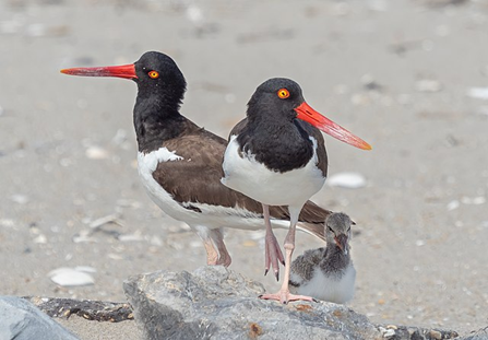
Figure 7: The American oystercatcher Haematopus palliatus survives almost exclusively on shellfish such as clams, oysters, and other molluscs. Rhododendrites, CC via Wikimedia Commons

Scientists are hoping to build up the population of this bird to 200 since they know the refuge can support this many individuals.  After doing some research, you learn that for every 50 birds, 30 birds are born annually and 22 birds die annually.  What is the population of 92 birds at the refuge expected to be next year?

First, let’s consider what information we have.  There is reference to a carrying capacity since we know the refuge can support 200 birds.  So K = 200.  We also know that the intrinsic growth rate, r, can be calculated with the data on birth rate and death rate.

If r = B – D    and we know that B = 30/50 or 0.60 and D = 22/50 or 0.44 we can calculate r

r = 0.6 – 0.44 or r = 0.16

Now, we choose the best population growth equation to use.  Since we have the carrying capacity, we will use the logistic equation

dN/dt = rN X [(K-N)/K]     with N = 92

dN/dt = (0.16)(92) X [(200-92)/200]

dN/dt = 14.72 X (108/200)

dN/dt = 14.72 X 0.54

dN/dt = 7.95 → round up to 8 birds

This means we expect the population of birds to CHANGE (dN) by 8 over 1 year (dt).  So to estimate the population number for next year we will add 8 to 92

8 + 92 = 100 birds for next year  (this is the answer)

Example #2

You are studying a population of an agricultural pest that has been introduced to a local farm.  Because there are no known predators of this pest species, its population is growing quickly and without any trace of slowing down.  You worry its population will decimate the crops and want to know what it’s population will be in 5 years.  Your sampling of the pest population gives you an estimate of 234 individuals.  You learn that its intrinsic growth rate is 0.34.  What is the population expected to be in 5 years?

We know that N=234 and r=0.34.  We don’t have any information about a carrying capacity (in fact, it appears there is not one) and so we must default to the exponential growth equation.

The exponential growth equation dN/dt = rN is designed to look at population growth one interval at a time.  So we could plug in our numbers and find year and year change 5 times.  For example,

dN/dt = 0.34 X 234

dN/dt = 79.56 → round up to 80

So during the first year, we expect 80 more pests or 234 + 80 = 314

Then using the new population size of 314 = N we can calculate for year 2:

dN/dt = 0.34 X 314

dN/dt = 106.76 → round up to 107 new pests or 314 + 107 = 421

And so on… (you would do this three more times to get to year 5)

An easier way to approach this problem when you are looking at a block of time in the future is to use a variation of the exponential equation:

N_t = N₀e^rt

So the new N_t = 234e(^0.34)(5)

N_t = 234e^1.7

N_t = 234 X 5.47

N_t = 1,279.98 → round up to 1,280

The new population in 5 years is expected to be 1,280!!

Population Dynamics and Regulation

The logistic model of population growth, while valid in many natural populations and a useful model, is a simplification of real-world population dynamics. Implicit in the model is that the carrying capacity of the environment does not change, which is not the case. The carrying capacity varies annually. For example, some summers are hot and dry whereas others are cold and wet; in many areas, the carrying capacity during the winter is much lower than it is during the summer. Also, natural events such as earthquakes, volcanoes, and fires can alter an environment and hence its carrying capacity. Additionally, populations do not usually exist in isolation. They share the environment with other species, competing with them for the same resources (interspecific competition). These factors are also important to understanding how a specific population will grow.

Population growth is regulated in a variety of ways. These are grouped into density-dependent factors, in which the density of the population affects growth rate and mortality, and density-independent factors, which cause mortality in a population regardless of population density. Wildlife biologists, in particular, want to understand both types because this helps them manage populations and prevent extinction or overpopulation.

Density-Dependent Regulation

Most density-dependent factors are biological in nature and include predation, inter- and intraspecific competition, and parasites. Usually, the denser a population is, the greater its mortality rate. For example, during intra- and interspecific competition, the reproductive rates of the species will usually be lower, reducing their populations’ rate of growth. In addition, low prey density increases the mortality of its predator because it has more difficulty locating its food source. Also, when the population is denser, diseases spread more rapidly among the members of the population, which affect the mortality rate.

Density dependent regulation was studied in a natural experiment with wild donkey populations on two sites in Australia (Choquento 1991). On one site the population was reduced by a population control program; the population on the other site received no interference. The high-density plot was twice as dense as the low-density plot. From 1986 to 1987 the high-density plot saw no change in donkey density, while the low-density plot saw an increase in donkey density. The difference in the growth rates of the two populations was caused by mortality, not by a difference in birth rates. The researchers found that numbers of offspring birthed by each mother was unaffected by density. Growth rates in the two populations were different mostly because of juvenile mortality caused by the mother’s malnutrition due to scarce high-quality food in the dense population.  Figure 8 shows the difference in age-specific mortalities in the two populations.

Figure 8: The graph shows the age-specific mortality rates for wild donkeys from high- and low-density populations.  The juvenile mortality is much higher in the high-density population because of maternal malnutrition caused by a shortage of high-quality food.

Density-Independent Regulation

Many factors that are typically physical in nature cause mortality of a population regardless of its density. These factors include weather, natural disasters, and pollution. An individual deer will be killed in a forest fire regardless of how many deer happen to be in that area. Its chances of survival are the same whether the population density is high or low. The same holds true for cold winter weather.

In real-life situations, population regulation is very complicated and density-dependent and independent factors can interact. A dense population that suffers mortality from a density-independent cause will be able to recover differently than a sparse population. For example, a population of deer affected by a harsh winter will recover faster if there are more deer remaining to reproduce.

Summary

Populations, groups of organisms of the same species, are found distributed throughout nature in different ways: uniform, clumped, and random.  Populations can also grow and change in different ways: exponentially or logistically.  The most common type of population growth is logistic, where populations grow until their carrying capacity is reached.  Once this maximum number is obtained, the population may stabilize at the carrying capacity or it may bounce up and under it.  If a population shoots over the carrying capacity by a lot, it will likely crash and you may likely see a local extinction as a result.  Ecologists use population models and mathematical equations to study how populations change over time and use these equations to predict what will happen over time.  In this way, we can make conservation decisions and management decisions to best suit our needs.

Sometimes the decisions made are based not only on the mathematical predictions, but also take into account environmental factors, like whether or not the population is controlled by density-dependent factors or not.  If something like food or nest boxes, density-dependent factors, influence populations, scientists can add or supplement to populations to help with population regulation.  Additionally, species have different intrinsic characteristics that may influence their population growth rates.  For example, species we call K-selected have a lower fecundity and take longer to become sexually mature compared to species we call r-selected which tend to mature quickly and produce many offspring at a time.  In this sense, r-selected populations can grow more quickly than K-selected populations.

Questions

Glossary

References

Choquenot, D. 1991. Density-Dependent Growth, Body Condition, and Demography in Feral Donkeys: Testing the Food Hypothesis. Ecology 72(3): 805-813.

Jones, C. 2022. All population text with the exception of “Problem Solving”.  Biology and the Citizen.  Utah State University.

Kosal, E. 2023. Problem Solving, K-selected and r-selected species, and Summary. NC State University.