2.1 Polar Covalent Bonds and Electronegativity

Up to this point, we’ve treated chemical bonds as either ionic or covalent. The bond in sodium chloride, for instance, is ionic. Sodium transfers an electron to chlorine to produce Na+ and Cl– ions, which are held together in the solid by electrostatic attractions between unlike charges. The C–C bond in ethane, however, is covalent. The two bonding electrons are shared equally by the two equivalent carbon atoms, resulting in a symmetrical electron distribution in the bond. Most bonds, however, are neither fully ionic nor fully covalent but are somewhere between the two extremes. Such bonds are called polar covalent bonds, meaning that the bonding electrons are attracted more strongly by one atom than the other so that the electron distribution between atoms is not symmetrical (Figure 2.2).

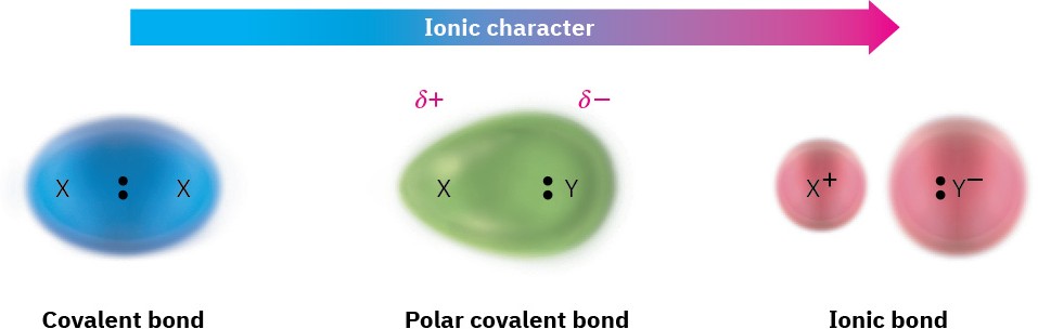
Figure 2.2 The continuum in bonding from covalent to ionic is a result of an unequal distribution of bonding electrons between atoms. The symbol δ (lowercase Greek letter delta) means partial charge, either partial positive (δ+) for the electron-poor atom or partial negative (δ–) for the electron-rich atom.

Bond polarity is due to differences in electronegativity (EN), the intrinsic ability of an atom to attract the shared electrons in a covalent bond. As shown in Figure 2.3, electronegativities are based on an arbitrary scale, with fluorine the most electronegative (EN = 4.0) and cesium the least (EN = 0.7). Metals on the left side of the periodic table attract electrons weakly and have lower electronegativities, while oxygen, nitrogen, and halogens on the right side of the periodic table attract electrons strongly and have higher electronegativities. Carbon, the most important element in organic compounds, has an intermediate electronegativity value of 2.5.

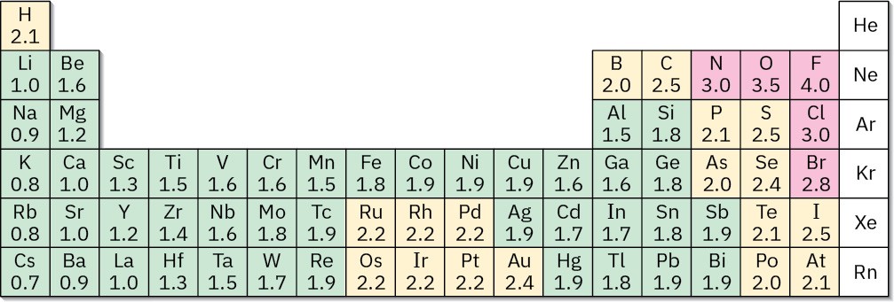
Figure 2.3 Electronegativity values and trends. Electronegativity generally increases from left to right across the periodic table and decreases from top to bottom. The values are on an arbitrary scale, with F = 4.0 and Cs = 0.7. Elements in red are the most electronegative, those in yellow are medium, and those in green are the least electronegative.

As a rough guide, bonds between atoms whose electronegativities differ by less than 0.5 are nonpolar covalent, bonds between atoms whose electronegativities differ by 0.5 to 2 are polar covalent, and bonds between atoms whose electronegativities differ by more than 2 are largely ionic. Carbon–hydrogen bonds, for example, are relatively nonpolar because carbon (EN = 2.5) and hydrogen (EN = 2.1) have similar electronegativities. Bonds between carbon and more electronegative elements such as oxygen (EN = 3.5) and nitrogen (EN = 3.0), by contrast, are polarized so that the bonding electrons are drawn away from carbon toward the electronegative atom. This leaves carbon with a partial positive charge, δ–, and the electronegative atom with a partial negative charge, δ–. An example is the C–O bond in methanol, CH3OH (Figure 2.4a). Bonds between carbon and less electronegative elements are polarized so that carbon bears a partial negative charge and the other atom bears a partial positive charge. An example is the C–Li bond in methyllithium, CH3Li (Figure 2.4b).

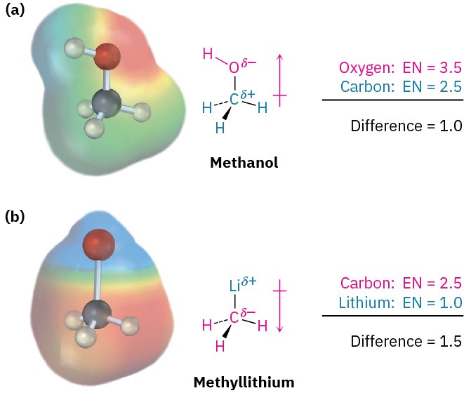
Figure 2.4 Polar covalent bonds. (a) Methanol, CH3OH, has a polar covalent C–O bond, and (b) methyllithium, CH3Li, has a polar covalent C–Li bond. The computer-generated representations, called electrostatic potential maps, use color to show calculated charge distributions, ranging from red (electron-rich; δ−) to blue (electron-poor; δ+).

Note in the representations of methanol and methyllithium in Figure 2.4 that a crossed arrowis used to indicate the direction of bond polarity. By convention, electrons are displaced in the direction of the arrow. The tail of the arrow (which looks like a plus sign) is electron-poor (δ+), and the head of the arrow is electron-rich (δ–).

Note also in Figure 2.4 that calculated charge distributions in molecules can be displayed visually with what are called electrostatic potential maps, which use color to indicate electron-rich (red; δ–) and electron-poor (blue; δ+) regions. In methanol, oxygen carries a partial negative charge and is colored red, while the carbon and hydrogen atoms carry partial positive charges and are colored blue-green. In methyllithium, lithium carries a partial positive charge (blue), while carbon and the hydrogen atoms carry partial negative charges (red). Electrostatic potential maps are useful because they show at a glance the electron-rich and electron-poor atoms in molecules. We’ll make frequent use of these maps throughout the text and will see many examples of how electronic structure correlates with chemical reactivity.

When speaking of an atom’s ability to polarize a bond, we often use the term inductive effect. An inductive effect is simply the shifting of electrons in a σ bond in response to the electronegativity of nearby atoms. Metals, such as lithium and magnesium, inductively donate electrons, whereas reactive nonmetals, such as oxygen and nitrogen, inductively withdraw electrons. Inductive effects play a major role in understanding chemical reactivity, and we’ll use them many times throughout this text to explain a variety of chemical observations.

Problem 2-1

Which element in each of the following pairs is more electronegative? (a)

Li or H (b)

B or Br (c)

Cl or I (d)

C or H Problem 2-2

Use the δ+/δ– convention to indicate the direction of expected polarity for each of the bonds indicated.

(a) H3C–Cl

(b)

H3C–NH2

(c)

H2N–H

(d) H3C–SH

(e)

H3C–MgBr

(f)

H3C–F

Problem 2-3

Use the electronegativity values shown in Figure 2.3 to rank the following bonds from least polar to most polar: H3C–Li, H3C–K, H3C–F, H3C–MgBr, H3C–OH

Problem 2-4

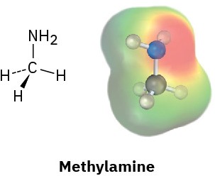
Look at the following electrostatic potential map of methylamine, a substance responsible for the odor of rotting fish, and tell the direction of polarization of the C–N bond: